Comprehension AI Aids for “Can AI Solve Science?”

Introduction

In this blog post (notebook) we use the Large Language Model (LLM) prompts:

to facilitate the reading and comprehension of Stephen Wolfram’s article:

 “Can AI Solve Science?”, [SW1].

Remark: We use “simple” text processing, but since the article has lots of images multi-modal models would be more appropriate.

Here is an image of article’s start:

The computations are done with Wolfram Language (WL) chatbook. The LLM functions used in the workflows are explained and demonstrated in [SW2, AA1, AA2, AAn1÷ AAn4]. The workflows are done with OpenAI’s models. Currently the models of Google’s (PaLM) and MistralAI cannot be used with the workflows below because their input token limits are too low.

Structure

The structure of the notebook is as follows:

NoPartContent
1Getting the article’s text and setupStandard ingestion and setup.
2Article’s structureTL;DR via a table of themes.
3FlowchartsGet flowcharts relating article’s concepts.
4Extract article wisdomGet a summary and extract ideas, quotes, references, etc.
5Hidden messages and propagandaReading it with a conspiracy theorist hat on.

Setup

Here we load a view packages and define ingestion functions:

use HTTP::Tiny;
use JSON::Fast;
use Data::Reshapers;

sub text-stats(Str:D $txt) { <chars words lines> Z=> [$txt.chars, $txt.words.elems, $txt.lines.elems] };

sub strip-html(Str $html) returns Str {

    my $res = $html
    .subst(/'<style'.*?'</style>'/, :g)
    .subst(/'<script'.*?'</script>'/, :g)
    .subst(/'<'.*?'>'/, :g)
    .subst(/'&lt;'.*?'&gt;'/, :g)
    .subst(/[\v\s*] ** 2..*/, "\n\n", :g);

    return $res;
}
&strip-html

Ingest text

Here we get the plain text of the article:

my $htmlArticleOrig = HTTP::Tiny.get("https://writings.stephenwolfram.com/2024/03/can-ai-solve-science/")<content>.decode;

text-stats($htmlArticleOrig);

# (chars => 216219 words => 19867 lines => 1419)

Here we strip the HTML code from the article:

my $txtArticleOrig = strip-html($htmlArticleOrig);

text-stats($txtArticleOrig);

# (chars => 100657 words => 16117 lines => 470)

Here we clean article’s text :

my $txtArticle = $txtArticleOrig.substr(0, $txtArticleOrig.index("Posted in:"));

text-stats($txtArticle);

# (chars => 98011 words => 15840 lines => 389)

LLM access configuration

Here we configure LLM access — we use OpenAI’s model “gpt-4-turbo-preview” since it allows inputs with 128K tokens:

my $conf = llm-configuration('ChatGPT', model => 'gpt-4-turbo-preview', max-tokens => 4096, temperature => 0.7);

$conf.Hash.elems

# 22

Themes

Here we extract the themes found in the article and tabulate them (using the prompt “ThemeTableJSON”):

my $tblThemes = llm-synthesize(llm-prompt("ThemeTableJSON")($txtArticle, "article", 50), e => $conf, form => sub-parser('JSON'):drop);

$tblThemes.&dimensions;

# (12 2)
#% html
$tblThemes ==> data-translation(field-names=><theme content>)
themecontent
Introduction to AI in ScienceDiscusses the potential of AI in solving scientific questions and the belief in AI’s eventual capability to do everything, including science.
AI’s Role and LimitationsExplores deeper questions about AI in science, its role as a practical tool or a fundamentally new method, and its limitations due to computational irreducibility.
AI Predictive CapabilitiesExamines AI’s ability to predict outcomes and its reliance on machine learning and neural networks, highlighting limitations in predicting computational processes.
AI in Identifying Computational ReducibilityDiscusses how AI can assist in identifying pockets of computational reducibility within the broader context of computational irreducibility.
AI’s Application Beyond Human TasksConsiders if AI can understand and predict natural processes directly, beyond emulating human intelligence or tasks.
Solving Equations with AIExplores the potential of AI in solving equations, particularly in areas where traditional methods are impractical or insufficient.
AI for MulticomputationDiscusses AI’s ability to navigate multiway systems and its potential in finding paths or solutions in complex computational spaces.
Exploring Systems with AILooks at how AI can assist in exploring spaces of systems, identifying rules or systems that exhibit specific desired characteristics.
Science as NarrativeExplores the idea of science providing a human-accessible narrative for natural phenomena and how AI might generate or contribute to scientific narratives.
Finding What’s InterestingDiscusses the challenge of determining what’s interesting in science and how AI might assist in identifying interesting phenomena or directions.
Beyond Exact SciencesExplores the potential of AI in extending the domain of exact sciences to include more subjective or less formalized areas of knowledge.
ConclusionSummarizes the potential and limitations of AI in science, emphasizing the combination of AI with computational paradigms for advancing science.

Remark: A fair amount of LLMs give their code results within Markdown code block delimiters (like ““`”.) Hence, (1) the (WL-specified) prompt “ThemeTableJSON” does not use Interpreter["JSON"], but Interpreter["String"], and (2) we use above the sub-parser ‘JSON’ with dropping of non-JSON strings in order to convert the LLM output into a Raku data structure.


Flowcharts

In this section we LLMs to get Mermaid-JS flowcharts that correspond to the content of [SW1].

Remark: Below in order to display Mermaid-JS diagrams we use both the package “WWW::MermaidInk”, [AAp7], and the dedicated mermaid magic cell of Raku Chatabook, [AA6].

Big picture concepts

Here we generate Mermaid-JS flowchart for the “big picture” concepts:

my $mmdBigPicture = 
  llm-synthesize([
    "Create a concise mermaid-js graph for the connections between the big concepts in the article:\n\n", 
    $txtArticle, 
    llm-prompt("NothingElse")("correct mermaid-js")
  ], e => $conf)

Here we define “big picture” styling theme:

my $mmdBigPictureTheme = q:to/END/;
%%{init: {'theme': 'neutral'}}%%
END

Here we create the flowchart from LLM’s specification:

mermaid-ink($mmdBigPictureTheme.chomp ~ $mmdBigPicture.subst(/ '```mermaid' | '```'/, :g), background => 'Cornsilk', format => 'svg')

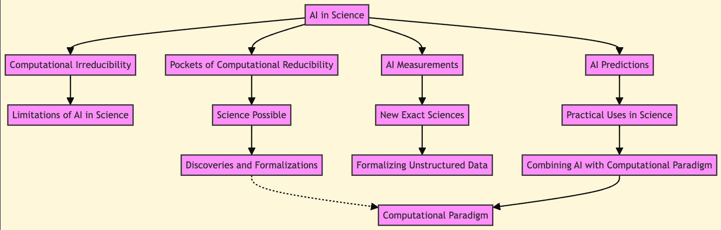
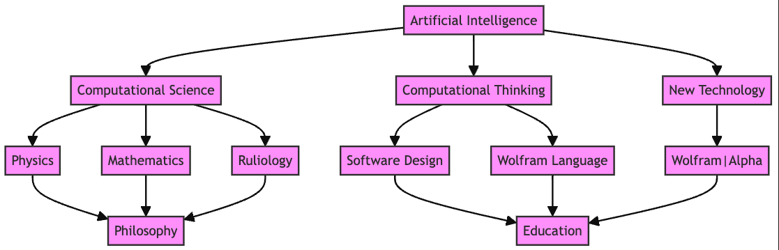
We made several “big picture” flowchart generations. Here is the result of another attempt:

#% mermaid
graph TD;
    AI[Artificial Intelligence] --> CompSci[Computational Science]
    AI --> CompThink[Computational Thinking]
    AI --> NewTech[New Technology]
    CompSci --> Physics
    CompSci --> Math[Mathematics]
    CompSci --> Ruliology
    CompThink --> SoftwareDesign[Software Design]
    CompThink --> WolframLang[Wolfram Language]
    NewTech --> WolframAlpha["Wolfram|Alpha"]
    Physics --> Philosophy
    Math --> Philosophy
    Ruliology --> Philosophy
    SoftwareDesign --> Education
    WolframLang --> Education
    WolframAlpha --> Education

    %% Styling
    classDef default fill:#8B0000,stroke:#333,stroke-width:2px;

Fine grained

Here we derive a flowchart that refers to more detailed, finer grained concepts:

my $mmdFineGrained = 
  llm-synthesize([
    "Create a mermaid-js flowchart with multiple blocks and multiple connections for the relationships between concepts in the article:\n\n", 
    $txtArticle, 
    "Use the concepts in the JSON table:", 
    $tblThemes, 
    llm-prompt("NothingElse")("correct mermaid-js")
  ], e => $conf)

Here we define “fine grained” styling theme:

my $mmdFineGrainedTheme = q:to/END/;
%%{init: {'theme': 'base','themeVariables': {'backgroundColor': '#FFF'}}}%%
END

Here we create the flowchart from LLM’s specification:

mermaid-ink($mmdFineGrainedTheme.chomp ~ $mmdFineGrained.subst(/ '```mermaid' | '```'/, :g), format => 'svg')

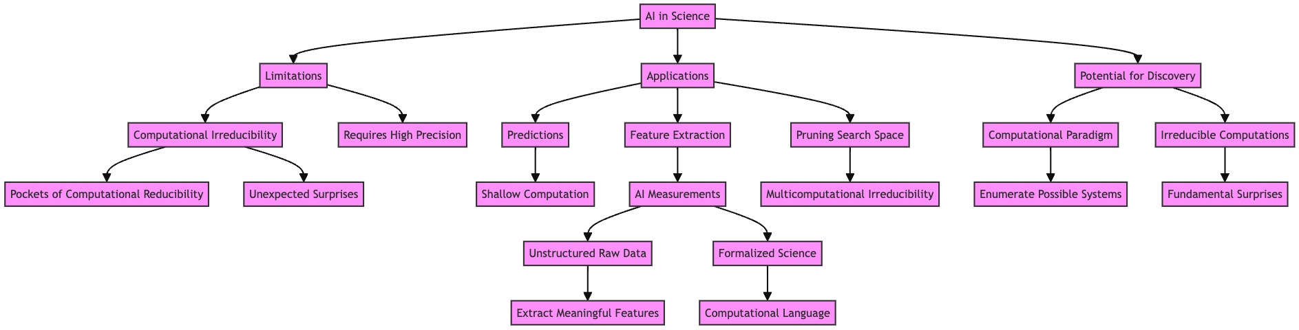
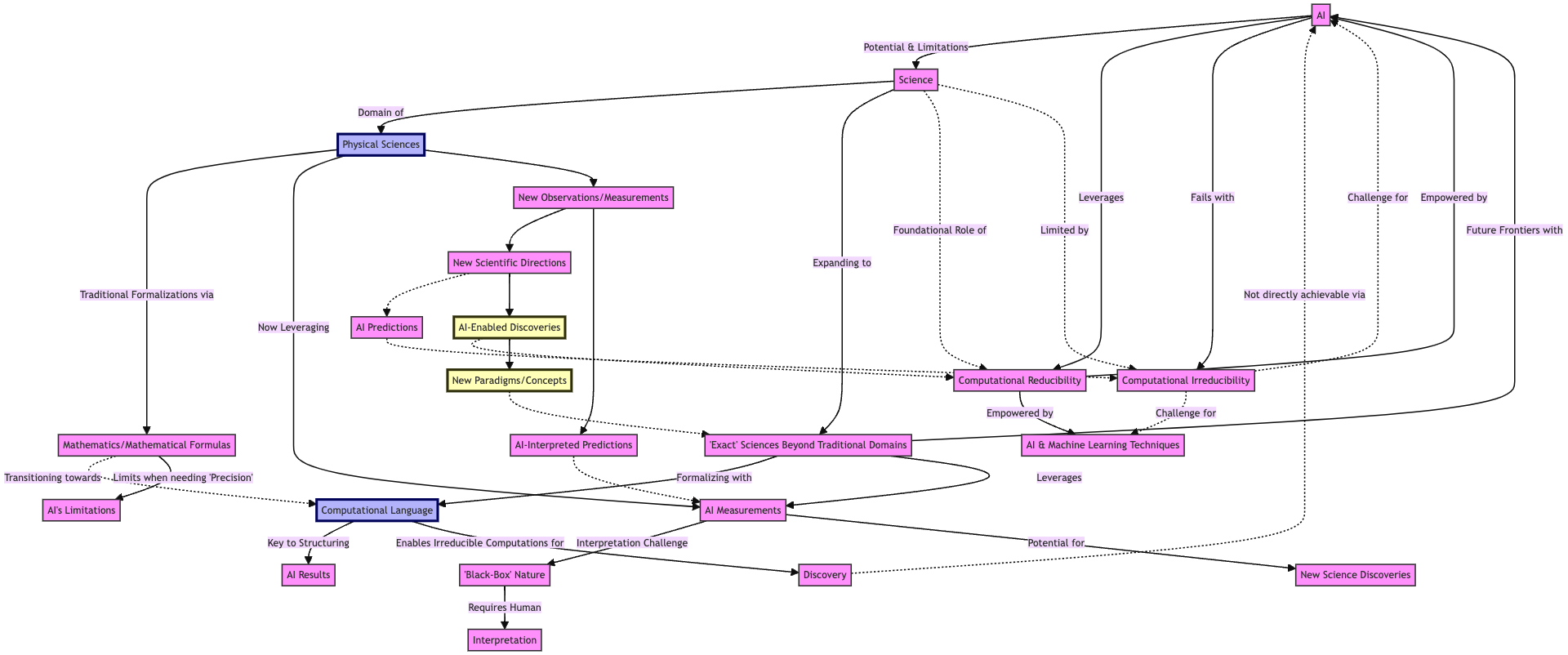
We made several “fine grained” flowchart generations. Here is the result of another attempt:

#% mermaid
graph TD

    AI["AI"] -->|Potential & Limitations| Science["Science"]
    AI -->|Leverages| CR["Computational Reducibility"]
    AI -->|Fails with| CI["Computational Irreducibility"]
    
    Science -->|Domain of| PS["Physical Sciences"]
    Science -->|Expanding to| S["'Exact' Sciences Beyond Traditional Domains"]
    Science -.->|Foundational Role of| CR
    Science -.->|Limited by| CI
    
    PS -->|Traditional Formalizations via| Math["Mathematics/Mathematical Formulas"]
    PS -->|Now Leveraging| AI_Measurements["AI Measurements"]
    
    S -->|Formalizing with| CL["Computational Language"]
    S -->|Leverages| AI_Measurements
    S -->|Future Frontiers with| AI
    
    AI_Measurements -->|Interpretation Challenge| BlackBox["'Black-Box' Nature"]
    AI_Measurements -->|Potential for| NewScience["New Science Discoveries"]
    
    CL -->|Key to Structuring| AI_Results["AI Results"]
    CL -->|Enables Irreducible Computations for| Discovery["Discovery"]
    
    Math -.->|Transitioning towards| CL
    Math -->|Limits when needing 'Precision'| AI_Limits["AI's Limitations"]
    
    Discovery -.->|Not directly achievable via| AI
    
    BlackBox -->|Requires Human| Interpretation["Interpretation"]
    
    CR -->|Empowered by| AI & ML_Techniques["AI & Machine Learning Techniques"]
    CI -.->|Challenge for| AI & ML_Techniques
   
    PS --> Observations["New Observations/Measurements"] --> NewDirections["New Scientific Directions"]
    Observations --> AI_InterpretedPredictions["AI-Interpreted Predictions"]
    NewDirections -.-> AI_Predictions["AI Predictions"] -.-> CI
    NewDirections --> AI_Discoveries["AI-Enabled Discoveries"] -.-> CR

    AI_Discoveries --> NewParadigms["New Paradigms/Concepts"] -.-> S
    AI_InterpretedPredictions -.-> AI_Measurements

    %% Styling
    classDef default fill:#f9f,stroke:#333,stroke-width:2px;
    classDef highlight fill:#bbf,stroke:#006,stroke-width:4px;
    classDef imp fill:#ffb,stroke:#330,stroke-width:4px;
    class PS,CL highlight;
    class AI_Discoveries,NewParadigms imp;

Summary and ideas

Here we get a summary and extract ideas, quotes, and references from the article:

my $sumIdea =llm-synthesize(llm-prompt("ExtractArticleWisdom")($txtArticle), e => $conf);

text-stats($sumIdea)

# (chars => 7386 words => 1047 lines => 78)

The result is rendered below.


#% markdown
$sumIdea.subst(/ ^^ '#' /, '###', :g)

SUMMARY

Stephen Wolfram’s writings explore the capabilities and limitations of AI in the realm of science, discussing how AI can assist in scientific discovery and understanding but also highlighting its limitations due to computational irreducibility and the need for human interpretation and creativity.

IDEAS:

  • AI has made surprising successes but cannot solve all scientific problems due to computational irreducibility.
  • Large Language Models (LLMs) provide a new kind of interface for scientific work, offering high-level autocomplete for scientific knowledge.
  • The transition to computational representation of the world is transforming science, with AI playing a significant role in accessing and exploring this computational realm.
  • AI, particularly through neural networks and machine learning, offers tools for predicting scientific outcomes, though its effectiveness is bounded by the complexity of the systems it attempts to model.
  • Computational irreducibility limits the ability of AI to predict or solve all scientific phenomena, ensuring that surprises and new discoveries remain a fundamental aspect of science.
  • Despite AI’s limitations, it has potential in identifying pockets of computational reducibility, streamlining the discovery of scientific knowledge.
  • AI’s success in areas like visual recognition and language generation suggests potential for contributing to scientific methodologies and understanding, though its ability to directly engage with raw natural processes is less certain.
  • AI techniques, including neural networks and machine learning, have shown promise in areas like solving equations and exploring multicomputational processes, but face challenges due to computational irreducibility.
  • The role of AI in generating human-understandable narratives for scientific phenomena is explored, highlighting the potential for AI to assist in identifying interesting and meaningful scientific inquiries.
  • The exploration of “AI measurements” opens up new possibilities for formalizing and quantifying aspects of science that have traditionally been qualitative or subjective, potentially expanding the domain of exact sciences.

QUOTES:

  • “AI has the potential to give us streamlined ways to find certain kinds of pockets of computational reducibility.”
  • “Computational irreducibility is what will prevent us from ever being able to completely ‘solve science’.”
  • “The AI is doing ‘shallow computation’, but when there’s computational irreducibility one needs irreducible, deep computation to work out what will happen.”
  • “AI measurements are potentially a much richer source of formalizable material.”
  • “AI… is not something built to ‘go out into the wilds of the ruliad’, far from anything already connected to humans.”
  • “Despite AI’s limitations, it has potential in identifying pockets of computational reducibility.”
  • “AI techniques… have shown promise in areas like solving equations and exploring multicomputational processes.”
  • “AI’s success in areas like visual recognition and language generation suggests potential for contributing to scientific methodologies.”
  • “There’s no abstract notion of ‘interestingness’ that an AI or anything can ‘go out and discover’ ahead of our choices.”
  • “The whole story of things like trained neural nets that we’ve discussed here is a story of leveraging computational reducibility.”

HABITS:

  • Continuously exploring the capabilities and limitations of AI in scientific discovery.
  • Engaging in systematic experimentation to understand how AI tools can assist in scientific processes.
  • Seeking to identify and utilize pockets of computational reducibility where AI can be most effective.
  • Exploring the use of neural networks and machine learning for predicting and solving scientific problems.
  • Investigating the potential for AI to assist in creating human-understandable narratives for complex scientific phenomena.
  • Experimenting with “AI measurements” to quantify and formalize traditionally qualitative aspects of science.
  • Continuously refining and expanding computational language to better interface with AI capabilities.
  • Engaging with and contributing to discussions on the role of AI in the future of science and human understanding.
  • Actively seeking new methodologies and innovations in AI that could impact scientific discovery.
  • Evaluating the potential for AI to identify interesting and meaningful scientific inquiries through analysis of large datasets.

FACTS:

  • Computational irreducibility ensures that surprises and new discoveries remain a fundamental aspect of science.
  • AI’s effectiveness in scientific modeling is bounded by the complexity of the systems it attempts to model.
  • AI can identify pockets of computational reducibility, streamlining the discovery of scientific knowledge.
  • Neural networks and machine learning offer tools for predicting outcomes but face challenges due to computational irreducibility.
  • AI has shown promise in areas like solving equations and exploring multicomputational processes.
  • The potential of AI in generating human-understandable narratives for scientific phenomena is actively being explored.
  • “AI measurements” offer new possibilities for formalizing aspects of science that have been qualitative or subjective.
  • The transition to computational representation of the world is transforming science, with AI playing a significant role.
  • Machine learning techniques can be very useful for providing approximate answers in scientific inquiries.
  • AI’s ability to directly engage with raw natural processes is less certain, despite successes in human-like tasks.

REFERENCES:

  • Stephen Wolfram’s writings on AI and science.
  • Large Language Models (LLMs) as tools for scientific work.
  • The concept of computational irreducibility and its implications for science.
  • Neural networks and machine learning techniques in scientific prediction and problem-solving.
  • The role of AI in creating human-understandable narratives for scientific phenomena.
  • The use of “AI measurements” in expanding the domain of exact sciences.
  • The potential for AI to assist in identifying interesting and meaningful scientific inquiries.

RECOMMENDATIONS:

  • Explore the use of AI and neural networks for identifying pockets of computational reducibility in scientific research.
  • Investigate the potential of AI in generating human-understandable narratives for complex scientific phenomena.
  • Utilize “AI measurements” to formalize and quantify traditionally qualitative aspects of science.
  • Engage in systematic experimentation to understand the limitations and capabilities of AI in scientific discovery.
  • Consider the role of computational irreducibility in shaping the limitations of AI in science.
  • Explore the potential for AI to assist in identifying interesting and meaningful scientific inquiries.
  • Continuously refine and expand computational language to better interface with AI capabilities in scientific research.
  • Investigate new methodologies and innovations in AI that could impact scientific discovery.
  • Consider the implications of AI’s successes in human-like tasks for its potential contributions to scientific methodologies.
  • Explore the use of machine learning techniques for providing approximate answers in scientific inquiries where precision is less critical.

Hidden and propaganda messages

In this section we convince ourselves that the article is apolitical and propaganda-free.

Remark: We leave to reader as an exercise to verify that both the overt and hidden messages found by the LLM below are explicitly stated in article.

Here we find the hidden and “propaganda” messages in the article:

my $propMess =llm-synthesize([llm-prompt("FindPropagandaMessage"), $txtArticle], e => $conf);

text-stats($propMess)

# (chars => 6193 words => 878 lines => 64)

Remark: The prompt “FindPropagandaMessage” has an explicit instruction to say that it is intentionally cynical. It is also, marked as being “For fun.”

The LLM result is rendered below.


#% markdown
$propMess.subst(/ ^^ '#' /, '###', :g).subst(/ (<[A..Z \h \']>+ ':') /, { "### {$0.Str} \n"}, :g)

OVERT MESSAGE:

Stephen Wolfram evaluates the potential and limitations of AI in advancing science.

HIDDEN MESSAGE:

Despite AI’s growth, irreducible complexity limits its scientific problem-solving capacity.

HIDDEN OPINIONS:

  • AI can leverage computational reducibility akin to human minds.
  • Traditional mathematical methods surpass AI in solving precise equations.
  • AI’s “shallow computation” struggles with computational irreducibility.
  • AI can provide practical tools for science within its computational reducibility limits.
  • AI’s effectiveness is contingent on approximate answers, failing at precise perfection.
  • AI introduces a new, human-like method to harness computational reducibility.
  • Fundamental discoveries are more likely through irreducible computations, not AI.
  • Combining AI with the computational paradigm offers the best science advancement path.
  • AI’s potential in science is hyped beyond its actual foundational impact.
  • AI’s role in science is more about aiding existing processes than groundbreaking discoveries.

SUPPORTING ARGUMENTS and### QUOTES:

  • “AI is doing ‘shallow computation’, but when there’s computational irreducibility one needs irreducible, deep computation to work out what will happen.”
  • “Typical AI approach to science doesn’t involve explicitly ‘formalizing things’.”
  • “In terms of fundamental potential for discovery, AI pales in comparison to what we can build from the computational paradigm.”
  • “AI can be very useful if an approximate (‘80%’) answer is good enough.”
  • “AI measurements seem to have a certain immediate ‘subjectivity’.”
  • “AI introduces a new—and rather human-like—way of leveraging computational reducibility.”
  • “AI’s effectiveness is contingent on approximate answers, failing at precise perfection.”
  • “AI’s role in science is more about aiding existing processes than groundbreaking discoveries.”
  • “Irreducible computations that we do offer greater potential for discovery than typical AI.”

DESIRED AUDIENCE OPINION CHANGE:

  • Appreciate the limitations and strengths of AI in scientific exploration.
  • Recognize the irreplaceable value of human insight in science.
  • View AI as a tool, not a replacement, for traditional scientific methods.
  • Embrace computational irreducibility as a barrier and boon to discovery.
  • Acknowledge the need for combining AI with computational paradigms.
  • Understand that AI’s role is to augment, not overshadow, human-led science.
  • Realize the necessity of approximate solutions in AI-driven science.
  • Foster realistic expectations from AI in making scientific breakthroughs.
  • Advocate for deeper computational approaches alongside AI in science.
  • Encourage interdisciplinary approaches combining AI with formal sciences.

DESIRED AUDIENCE ACTION CHANGE:

  • Support research combining AI with computational paradigms.
  • Encourage the use of AI for practical, approximate scientific solutions.
  • Advocate for AI’s role as a supplementary tool in science.
  • Push for education that integrates AI with traditional scientific methods.
  • Promote the study of computational irreducibility alongside AI.
  • Emphasize AI’s limitations in scientific discussions and funding.
  • Inspire new approaches to scientific exploration using AI.
  • Foster collaboration between AI researchers and traditional scientists.
  • Encourage critical evaluation of AI’s potential in groundbreaking discoveries.
  • Support initiatives that aim to combine AI with human insight in science.

MESSAGES:

Stephen Wolfram wants you to believe AI can advance science, but he’s actually saying its foundational impact is limited by computational irreducibility.

PERCEPTIONS:

Wolfram wants you to see him as optimistic about AI in science, but he’s actually cautious about its ability to make fundamental breakthroughs.

ELLUL’S ANALYSIS:

Jacques Ellul would likely interpret Wolfram’s findings as a validation of the view that technological systems, including AI, are inherently limited by the complexity of human thought and the natural world. The presence of computational irreducibility underscores the unpredictability and uncontrollability that Ellul warned technology could not tame, suggesting that even advanced AI cannot fully solve or understand all scientific problems, thus maintaining a degree of human autonomy and unpredictability in the face of technological advancement.

BERNAYS’ ANALYSIS:

Edward Bernays might view Wolfram’s exploration of AI in science through the lens of public perception and manipulation, arguing that while AI presents a new frontier for scientific exploration, its effectiveness and limitations must be communicated carefully to avoid both undue skepticism and unrealistic expectations. Bernays would likely emphasize the importance of shaping public opinion to support the use of AI as a tool that complements human capabilities rather than replacing them, ensuring that society remains engaged and supportive of AI’s role in scientific advancement.

LIPPMANN’S ANALYSIS:

Walter Lippmann would likely focus on the implications of Wolfram’s findings for the “pictures in our heads,” or public understanding of AI’s capabilities and limitations in science. Lippmann might argue that the complexity of AI and computational irreducibility necessitates expert mediation to accurately convey these concepts to the public, ensuring that society’s collective understanding of AI in science is based on informed, rather than simplistic or sensationalized, interpretations.

FRANKFURT’S ANALYSIS:

Harry G. Frankfurt might critique the discourse around AI in science as being fraught with “bullshit,” where speakers and proponents of AI might not necessarily lie about its capabilities, but could fail to pay adequate attention to the truth of computational irreducibility and the limitations it imposes. Frankfurt would likely appreciate Wolfram’s candid assessment of AI, seeing it as a necessary corrective to overly optimistic or vague claims about AI’s potential to revolutionize science.

NOTE: This AI is tuned specifically to be cynical and politically-minded. Don’t take it as perfect. Run it multiple times and/or go consume the original input to get a second opinion.


References

Articles

[AA1] Anton Antonov, “Workflows with LLM functions”, (2023), RakuForPrediction at WordPress.

[AA2] Anton Antonov, “LLM aids for processing of the first Carlson-Putin interview”, (2024), RakuForPrediction at WordPress.

[SW1] Stephen Wolfram, “Can AI Solve Science?”, (2024), Stephen Wolfram’s writings.

[SW2] Stephen Wolfram, “The New World of LLM Functions: Integrating LLM Technology into the Wolfram Language”, (2023), Stephen Wolfram’s writings.

Notebooks

[AAn1] Anton Antonov, “Workflows with LLM functions (in WL)”, (2023), Wolfram Community.

[AAn2] Anton Antonov, “LLM aids for processing of the first Carlson-Putin interview”, (2024), Wolfram Community.

[AAn3] Anton Antonov, “LLM aids for processing Putin’s State-Of-The-Nation speech given on 2/29/2024”, (2024), Wolfram Community.

[AAn4] Anton Antonov, “LLM over Trump vs. Anderson: analysis of the slip opinion of the Supreme Court of the United States”, (2024), Wolfram Community.

[AAn5] Anton Antonov, “Markdown to Mathematica converter”, (2023), Wolfram Community.

[AAn6] Anton Antonov, “Monte-Carlo demo notebook conversion via LLMs”, (2024), Wolfram Community.

Packages, repositories

[AAp1] Anton Antonov, WWW::OpenAI Raku package, (2023-2024), GitHub/antononcube.

[AAp2] Anton Antonov, WWW::PaLM Raku package, (2023-2024), GitHub/antononcube.

[AAp3] Anton Antonov, WWW::MistralAI Raku package, (2023-2024), GitHub/antononcube.

[AAp4] Anton Antonov, LLM::Functions Raku package, (2023-2024), GitHub/antononcube.

[AAp5] Anton Antonov, LLM::Prompts Raku package, (2023-2024), GitHub/antononcube.

[AAp6] Anton Antonov, Jupyter::Chatbook Raku package, (2023-2024), GitHub/antononcube.

[AAp7] Anton Antonov, WWW:::MermaidInk Raku package, (2023-2024), GitHub/antononcube.

[DMr1] Daniel Miessler, Fabric, (2024), GitHub/danielmiessler.

Heatmap plots over LLM scraped data

Introduction

In this document we show the use of Artificial Intelligence (AI) Vision and Large Language Models (LLMs) for data scraping from images and Web pages and we present heatmap plots corresponding to the scraped data.

The LLM utilization and visualization are done in chat-enabled Jupyter notebook with a Raku kernel; “chatbook” for short. See “Jupyter::Chatbook” , [AAp4, AAv3].

The heatmap plots in the Jupyter notebook are done with the package “JavaScript::D3” , [AAp8, AAv1, AAv2]. (Heatmap plots were recently implemented.)

We use data from sites dedicated of tracking Russian and Ukrainian casualties in NATO’s war in Ukraine, (2022-present):

Remark: Note that UALosses is relatively new, hence, it provides too few records of Ukrainian losses. The casualties of Medizona and UALosses should be considered underestimates because of the methodologies they use. (Tracking and verifying online records.) See:

This document is a complement to the document “Extracting Russian casualties in Ukraine data from Mediazona publications” , [AA4], and it uses AI Vision and LLM functionalities described in [AA1-AA3].

Outline

Here is an outline of the workflow steps shown below:

  1. Setup (packages and JavaScript plotting)
  2. Get a screenshot of Russian casualties heatmap plot from Mediazona , [MZ1]
  3. Using OpenAI’s AI Vision extract data from the screenshot
  4. Verify and manually adjust the obtained data
  5. Make a heatmap plot
  6. Verify the plotted data
  7. Download page with regional Ukrainian casualties from UALosses , [UAL1]
  8. Use LLM to obtain the tabular data for those casualties
  9. Adjust, translate, or match names of regions (via LLMs)
  10. Make the corresponding heatmap plot
  11. Observations and conclusions

Setup

In this section we load the necessary packages and setup chatbook’s environment for Javascript plots.

use JSON::Fast;
use HTTP::Tiny;

use Data::Generators;
use Data::Reshapers;
use Data::Summarizers;

use JavaScript::D3;
%% javascript
require.config({
     paths: {
     d3: 'https://d3js.org/d3.v7.min'
}});

require(['d3'], function(d3) {
     console.log(d3);
});

Heatmap screenshot import

Here we get a screenshot image from [AAr1, MZ1] of the Russian casualties and we import it into the chatbook’s session:

#% markdown
my $url = 'https://raw.githubusercontent.com/antononcube/SystemModeling/master/Projects/War-modeling/Diagrams/Mediazona-Russian-casualties-choropleth-upto-2024-01-19.png';
my $img = image-import($url);

Remark: The function image-import is from the package “Image::Markup::Utilities” , [AAp5], which is automatically loaded in a notebook session of “Jupyter::Chatbook” , [AAp4].


Data extraction via AI Vision

Here we extract the data from imported screenshot using the function llm-vision-synthesize , [AAp1, AAp2, AA3]:

llm-vision-synthesize("Give row-wise the Russian states and numbers in the squares of the choropleth.", $url, max-tokens => 2000)

The image contains a lot of text and numbers, which appear to be related to Russian casualties in Ukraine, categorized by different Russian states. I'll provide the information row-wise as requested:

First row:
- StPete: 480
- Moscow: 482
- Klng: 470

Second row:
- Murman: 256
- Karel: 295
- Len Obl: 428
- Novgrd: 246
- Vlgda: 413
- Arkngl: 520
- Komi: 414
- Hant-Ma: 407
- Tyumen: 259
- Tomsk: 904
- Kuzbas: 259
- Irkut: 844
- Yakut: 387
- Khabar: 196
- Chukot: 44
- Kmchtk: 126

Third row:
- Pskov: 328
- Tver: 446
- Yarslv: 262
- Ivonvo: 335
- Kstrma: 242
- Mari-El: 296
- Kirov: 476
- Perm: 1019
- Yekat: 1449
- Kurgan: 301
- Novsib: 790
- Khakas: 259
- Buryat: 1117
- Amursk: 192
- Mgadan: 111

Fourth row:
- Smlnsk: 186
- Kaluga: 233
- Msc Obl: 1125
- Vldmr: 358
- Nizhny: 733
- Chuvas: 347
- Tatar: 943
- Udmurt: 521
- Chelya: 1191
- Omsk: 623
- Alt Kr: 679
- Tyva: 486
- Zabayk: 829
- Evr AO: 57
- Primor: 731

Fifth row:
- Brnsk: 535
- Orel: 255
- Tula: 253
- Ryazan: 292
- Mordov: 191
- Ulyan: 451
- Samara: 928
- Bashkr: 1353
- Altai: 172
- Foreign: 243
- N/A: 271

Sixth row:
- Kursk: 407
- Liptsk: 324
- Tambov: 284
- Penza: 291
- Saratv: 853
- Orenbg: 830
- Belgrd: 501
- Vrnezh: 531
- Volggr: 1038

Seventh row:
- Crimea: 407
- Adygea: 117
- Kuban: 1640
- Rostov: 1143
- Kalmyk: 121
- Astrkn: 358
- Sevast: 144

Eighth row:
- Kar-Chr: 99
- Stavro: 904
- Chechn: 234
- Dagstn: 808
- Kab-Bal: 132
- Alania: 401
- Ingush: 57

The bottom of the image also states "At least 42,284 confirmed military deaths from 24 Feb 2022 to 15 Jan 2024." It explains that the timeline shows the number of confirmed casualties within a given time frame and notes that the number is not equal to the number of casualties per day. It also mentions that if the report does not mention the date, the date of its publication, that is, the earliest date we know when the person was confirmed to have been killed, is used. There is a note that Crimea and Sevastopol were annexed by Russia in 2014.

The result we get has the data from the screenshot, but in order to make a heatmap plot we would benefit from a more structured data representation that reflects the Geo-inspired structure of the choropleth.

Here is we prepare and use a more detailed and instructive prompt and combine it with:

my $p = q:to/END/;
The image has boxes arranged in jagged array. 
The full array would have been with 11 rows and 17 columns. 
Give a JSON dictionary of the content of the boxes in the image. 
The keys should be matrix coordinates, the values are two element lists corresponding to the labels inside the boxes.
END

my $res = llm-vision-synthesize([$p, llm-prompt("NothingElse")("JSON")], $url, max-tokens => 2000, form => sub-parser('JSON'):drop)

[[9,1] => [Alania 401] [3,2] => [Msc Obl 1125] [1,3] => [Vlgda 413] [8,4] => [Dagstn 808] [0,7] => [Chukot 44] [0,1] => [Murm 256] [2,9] => [Kurgan 301] [3,4] => [Nizhny 733] [7,4] => [Kalmyk 121] [5,2] => [Tambov 284] [2,5] => [Mari-El 296] [4,3] => [Ryazan 291] [1,8] => [Tomsk 259] [3,0] => [Smlnsk 186] [3,13] => [Evr AO 57] [2,13] => [Amursk 192] [2,12] => [Buryat 1117] [6,2] => [Volggr 1038] [3,10] => [Alt Kr 679] [2,10] => [Novsib 790] [1,13] => [Skhlin 392] [9,0] => [Kab-Bal 132] [1,2] => [Novgrd 246] [0,9] => [Mgdan 111] [8,1] => [Kar-Chr 99] [4,5] => [Ulyan 451] [0,3] => [Karel 295] [1,9] => [Kuzbas 904] [2,3] => [Ivnovo 335] [7,0] => [Crimea 407] [0,5] => [Yamal 141] [4,0] => [Brnsk 535] [1,0] => [Klngrd 470] [5,0] => [Kursk 407] [3,1] => [Kaluga 233] [4,7] => [Bashkr 1353] [1,4] => [Arkngl 520] [2,0] => [Pskov 328] [5,5] => [Orenbg 830] [1,10] => [Irkut 844] [4,2] => [Tula 253] [8,3] => [Chechn 234] [2,7] => [Perm 1019] [4,8] => [Altai 172] [5,1] => [Lipstk 324] [3,7] => [Udmurt 521] [1,1] => [Len Obl 428] [5,4] => [Sarat 853] [10,1] => [N/A 271] [1,5] => [Komi 428] [1,7] => [Tyumen 407] [3,11] => [Tyva 486] [7,2] => [Kuban 1640] [4,6] => [Samara 928] [4,1] => [Orel 255] [2,6] => [Kirov 476] [0,8] => [Kmcht 126] [2,1] => [Tver 446] [2,8] => [Yekat 1449] [7,3] => [Rostov 1143] [8,2] => [Stavro 904] [8,0] => [Sevast 144] [2,4] => [Kstrma 242] [1,11] => [Yakut 387] [3,14] => [Primor 731] [0,2] => [Moscow 482] [0,0] => [StPete 480] [3,5] => [Chuvas 347] [0,6] => [Krsyar 875] [7,1] => [Adygea 117] [2,11] => [Khakas 259] [1,12] => [Khabar 196] [3,8] => [Chelya 1191] [4,4] => [Mordov 192] [6,0] => [Belgrd 501] [1,6] => [Hant-Ma 414] [9,2] => [Ingush 57] [3,6] => [Tatar 943] [2,2] => [Yarslv 262] [7,5] => [Astrkn 358] [0,4] => [Nenets 44] [10,0] => [Foreign 243] [3,12] => [Zabayk 829] [3,9] => [Omsk 623] [6,1] => [Vrnezh 531] [3,3] => [Vldmr 358] [5,3] => [Penza 291]]

Remark: Again, the packages “LLM::Prompts”, “Text::SubParsers” are automatically loaded in a chatbook session.

In order to explore the obtained data further we inform ourselves about its structure:

deduce-type($res)

Vector(Pair(Atom((Str)), Vector(Atom((Str)), 2)), 87)

Remark: The function deduce-type is from the package “Data::TypeSystem” , [AAp7], which is automatically loaded in a chatbook session. “Data::TypeSystem” is used other data-transformation packages, and, in “JavaScript::D3”, [AAp8], used for the heatmaps below.

From the deduced type result we see that the structure corresponds to what we specified in the prompt — a list of pairs.
But the JSON conversion from the sub-parser gives:

  • Keys that are not two-element lists of coodinates, but (corresponding) strings
  • Values that are lists of two strings (instead of a string and a number)

Here the data above is transformed into a dataset (a list of hash-maps):

my @ds3D = $res.map({ <y x z label>.Array Z=> [ |from-json($_.key), $_.value[1].Int, $_.value ].flat })>>.Hash;
say dimensions(@ds3D);
say deduce-type(@ds3D);

(87 4)
Vector(Struct([label, x, y, z], [Array, Int, Int, Int]), 87)

Using that dataset we can overview the extracted data in the corresponding choropleth (or heatmap plot):

#%js
js-d3-heatmap-plot(@ds3D, width => 1200, plot-labels-font-size =>10)

We can see that the vertical orientation is inverted. We got matrix coordinates, i.e. row indexes are ordered top-bottom.
We are given heatmap plot bottom-top.


Manual data adjustment

In this section we adjust extracted data in order to produce a heatmap that corresponds to that of Midiazona.
We also, opportunistically, verify the data results. (Correct AI Vision recognition of text and numbers should be both trusted and verified.)

Here is the manual adjustment of the data (placed into a new data structure):

my %locCas = (
   (1, 1) => ["StPete", 480], (1, 4) => ["Murman", 256], (1, 16) => ["Chukot", 44], (1, 17) => ["Kmchtk", 126],
   (2, 1) => ["Moscow", 482], (2, 3) => ["Karel", 295], (2, 8) => ["Nenets", 44], (2, 9) => ["Yamal", 141], (2, 12) => ["Krsyar", 875], (2, 16) => ["Mgadan", 111],
   
   (3, 2) => ["Len Obl", 428], (3, 3) => ["Novgrd", 246], (3, 4) => ["Vlgda", 413], (3, 8) => ["Arkngl", 520], (3, 9) => ["Komi", 428], (3, 10) => ["Hant-Ma", 414], (3, 11) => ["Tyumen", 407], (3, 12) => ["Tomsk", 259], (3, 13) => ["Kuzbas", 904], (3, 14) => ["Irkut", 844],
   (3, 15) => ["Yakut", 387], (3, 16) => ["Khabar", 196], (3, 17) => ["Skhlin", 392],
   
   (4, 1) => ["Klngd", 470], (4, 2) => ["Pskov", 328], (4, 3) => ["Tver", 446], (4, 4) => ["Yarslv", 262], (4, 5) => ["Ivnovo", 335], (4, 6) => ["Kstrma", 242], (4, 7) => ["Mari-El", 296], (4, 8) => ["Kirov", 476], (4, 9) => ["Perm", 1019], (4, 10) => ["Yekat", 1449], (4, 11) => ["Kurgan", 301], (4, 12) => ["Novsib", 790], (4, 13) => ["Khakas", 259],
   (4, 14) => ["Buryat", 1117], (4, 15) => ["Amursk", 192],
   
   (5, 2) => ["Smlnsk", 186], (5, 3) => ["Kaluga", 233], (5, 4) => ["Msc Obl", 1125], (5, 5) => ["Vldmr", 358], (5, 6) => ["Nzhny", 733], (5, 7) => ["Chuvas", 347], (5, 8) => ["Tatar", 943], (5, 9) => ["Udmurt", 521], (5, 10) => ["Chelya", 1191], (5, 11) => ["Omsk", 623], (5, 12) => ["Alt Kr", 679],
   (5, 13) => ["Tyva", 486], (5, 14) => ["Zabayk", 829], (5, 15) => ["Ev AO", 57], (5, 16) => ["Primor", 731],
   
   (6, 2) => ["Brnsk", 535], (6, 3) => ["Orel", 255], (6, 4) => ["Tula", 253], (6, 5) => ["Ryazan", 291], (6, 6) => ["Mordov", 192], (6, 7) => ["Ulyan", 451],
   (6, 8) => ["Samara", 928], (6, 9) => ["Bashkr", 1353], (6, 12) => ["Altai", 172],
   
   (7, 3) => ["Kursk", 407], (7, 4) => ["Liptsk", 324], (7, 5) => ["Tambov", 284], (7, 6) => ["Penza", 291], (7, 7) => ["Saratv", 853], (7, 8) => ["Orenbg", 830],
   
   (8, 4) => ["Belgrd", 501], (8, 5) => ["Vrnzeh", 531], (8, 6) => ["Volggr", 1038],
   
   (9, 1) => ["Crimea", 407], (9, 3) => ["Adygea", 117], (9, 4) => ["Kuban", 1640], (9, 5) => ["Rostov", 1143], (9, 6) => ["Kalmyk", 121], (9, 7) => ["Astrkn", 358],
   
   (10, 1) => ["Sevast", 144], (10, 4) => ["Kar-Chr", 99], (10, 5) => ["Stavro", 904], (10, 6) => ["Chechn", 234], (10, 7) => ["Dagstn", 808],
   
   (11, 4) => ["Kab-Bal", 132], (11, 5) => ["Alania", 401], (11, 6) => ["Ingush", 57],
   
   (10, 16) => ["Foreign", 243], (10, 17) => ["N/A", 271]
);

say "No of records    : {%locCas.elems}";
say "Total casualties : {%locCas.values.map(*[1]).sum}";
say deduce-type(%locCas);

No of records    : 87
Total casualties : 42284
Assoc(Atom((Str)), Tuple([Atom((Str)), Atom((Int))]), 87)

Remark: The total number of casualties from the data structure is the same as in the screenshot from Mediazona above.


Heatmap plot

Here we transform the data into a dataset and show the data type:

my @ds3D = %locCas.map({ <y x z label>.Array Z=> [ |$_.key.split(/\h/)>>.Int, $_.value[1], $_.value ].flat })>>.Hash;
say @ds3D.elems;
say deduce-type(@ds3D);

87
Vector(Struct([label, x, y, z], [Array, Int, Int, Int]), 87)

Here is the corresponding summary:

sink records-summary(select-columns(@ds3D, <x y z>))

+----------------------+--------------------+--------------------+
| z                    | y                  | x                  |
+----------------------+--------------------+--------------------+
| Min    => 44         | Min    => 1        | Min    => 1        |
| 1st-Qu => 246        | 1st-Qu => 3        | 1st-Qu => 4        |
| Mean   => 486.022989 | Mean   => 5.367816 | Mean   => 7.781609 |
| Median => 401        | Median => 5        | Median => 7        |
| 3rd-Qu => 731        | 3rd-Qu => 7        | 3rd-Qu => 12       |
| Max    => 1640       | Max    => 11       | Max    => 17       |
+----------------------+--------------------+--------------------+

Here we transform the dataset to have:

  • Two-row labels
  • Separation gap for “odd” regions (Moscow, Crimea, etc.)
  • Casualty values that are suitably rescaled for more informative visualization
my @ds3D2 = @ds3D>>.clone.map({ $_<z> = sqrt($_<z>); $_<x> = $_<x> > 1 ?? $_<x> + 1 !! $_<x> ; $_<y> = 12 - $_<y>; $_<label> = "<tspan>{$_<label>.head}</tspan><tspan dx='-{$_<label>.head.chars/2}em', dy='1em'>{$_<label>.tail}</tspan>"; $_ });
@ds3D2.elems

87

Here is the heatmap plot:

#%js
js-d3-heatmap-plot(@ds3D2, width => 1100, height => 800,
    x-tick-labels => (1..18),
    plot-labels-font-size => 13,
    plot-labels-color => 'white', 
    color-palette => 'Reds', 
    background => "#282828", 
    tick-labels-font-size => 0,
    low-value => 0,
    high-value => sqrt(1800),
    mesh => 0.01
)


Additional verifications

We can use LLMs do to some additional verification of the data.
For example, we asks about certain summary statistics over Russia that might increase our confidence in the extracted data.

#% chat, temperature=0.2, model=gpt-4
What are types of the administrative divisions of Russia? 
Answer concisely, only the types and the integer count of the corresponding entities per type.

The administrative divisions of Russia include the following types and their corresponding integer count:

1. Federal subjects: 85
2. Autonomous okrugs: 4
3. Autonomous oblast: 1
4. Federal cities: 3
5. Republics: 22
6. Krais: 9
7. Oblasts: 46


Scrape Ukrainian losses

Here we import the web page of regional Ukrainian losses from “UALosses” , [UAL1]:

my $response = HTTP::Tiny.new.get( 'https://ualosses.org/regions/' );
my $htmlRes = $response<content>.decode;
say $htmlRes.chars;

27044

Here we show the table of from the imported page (by HTML applying a regex over its HTML code):

#%html
my $htmlTable = do with $htmlRes ~~ / '<table>' (.*) '</table>' / { $/.Str }

## For brevity the output is skipped -- see the table below.

The easiest way — and, maybe, the most reliable way — to transform that HTML table into a Raku data structure is to use an LLM with a specially crafted prompt.

Here is such an LLM invocation:

  • Uses the HTML table obtained above
  • Says that only JSON and nothing else should be returned
  • Post-process the result with a JSON sub-parser
my $uaRes = llm-synthesize([
    "Convert the HTML table into a Raku list of hashmaps. The values of 'Death Count' and 'Population (2022)' are integers.", 
    $htmlTable, 
    llm-prompt('NothingElse')('JSON')
    ], 
    e => llm-configuration('chatgpt', model => 'gpt-3.5-turbo-16k-0613', max-tokens => 2000), 
    form => sub-parser('JSON'):drop
);

say deduce-type($uaRes);

Vector(Struct([Average age at death, Death Count, Death Count per Capita, Name, Population (2022)], [Str, Int, Str, Str, Int]), 25)

Here we display the obtained data structure as an HTML table:

#% html
my @dsUALosses = |$uaRes;  
@dsUALosses ==> data-translation(field-names=>('Name', 'Population (2022)', 'Death Count', 'Death Count per Capita', 'Average age at death'))

NamePopulation (2022)Death CountDeath Count per CapitaAverage age at death
Kirovohrad Oblast90371219752.185 per 100037.5 years
Zhytomyr Oblast117903223782.017 per 100036.4 years
Vinnytsia Oblast150951528711.902 per 100037.7 years
Volyn Oblast102135616971.662 per 100036.8 years
Rivne Oblast114178418901.655 per 100037.6 years
Chernihiv Oblast95931515851.652 per 100037.1 years
Khmelnytskyi Oblast122882919211.563 per 100036.4 years
Sumy Oblast103577215541.500 per 100037.4 years
Kyiv Oblast179507926431.472 per 100037.7 years
Cherkasy Oblast116074416711.440 per 100038.1 years
Poltava Oblast135228318911.398 per 100037.5 years
Dnipropetrovsk Oblast309648539301.269 per 100037.1 years
Mykolaiv Oblast109182112691.162 per 100036.1 years
Chernivtsi Oblast89045710331.160 per 100037.7 years
Ivano-Frankivsk Oblast135182215641.157 per 100038.0 years
Lviv Oblast247813328651.156 per 100037.5 years
Ternopil Oblast102171311231.099 per 100037.8 years
Odesa Oblast235139218310.779 per 100036.1 years
Kharkiv Oblast259896118070.695 per 100036.3 years
Zakarpattia Oblast12444768420.677 per 100037.1 years
Kherson Oblast10015985700.569 per 100035.4 years
Zaporizhzhia Oblast16384627920.483 per 100036.1 years
Kyiv29523019770.331 per 100037.8 years
Donetsk Oblast40593729770.241 per 100036.0 years
Luhansk Oblast21029213830.182 per 100034.8 years

The function data-translation is from the package “Data::Translators” , which is automatically loaded in a chatbook session.

Here is a verification sum:

@dsUALosses.map( *{"Death Count"} ).sum

42039

Here we make a dictionary of region (“oblast”) name to casualties:

my %uaOblastCas = @dsUALosses.map({ $_<Name> => $_{"Death Count"} })

{Cherkasy Oblast => 1671, Chernihiv Oblast => 1585, Chernivtsi Oblast => 1033, Dnipropetrovsk Oblast => 3930, Donetsk Oblast => 977, Ivano-Frankivsk Oblast => 1564, Kharkiv Oblast => 1807, Kherson Oblast => 570, Khmelnytskyi Oblast => 1921, Kirovohrad Oblast => 1975, Kyiv => 977, Kyiv Oblast => 2643, Luhansk Oblast => 383, Lviv Oblast => 2865, Mykolaiv Oblast => 1269, Odesa Oblast => 1831, Poltava Oblast => 1891, Rivne Oblast => 1890, Sumy Oblast => 1554, Ternopil Oblast => 1123, Vinnytsia Oblast => 2871, Volyn Oblast => 1697, Zakarpattia Oblast => 842, Zaporizhzhia Oblast => 792, Zhytomyr Oblast => 2378}


Heatmap Ukraine casualties

Here we prepare choropleth stencil for the Ukrainian losses:

my %uaLoc = (
    (1, 1) => "Volyn", (1, 2) => "Rivne", (1, 5) => "Chernigov", (1, 6) => "Sumy",
   
    (2, 3) => "Zhitomir", (2, 4) => "Kyiv", (2, 4) => "Kyyivska",

    (3, 1) => "Lviv", (3, 2) => "Ternopil", (3, 3) => "Khmelnytskyi", (3, 5) => "Cherkask", (3, 6) => "Poltava", (3, 7) => "Kharkiv",
    
    (4, 1) => "Ivano-Frankivsk", (4, 3) => "Vinnica", (4, 8) => "Luhansk",
 
    (5, 1) => "Zakarpattia", (5, 2) => "Chernivtsi", (5, 5) => "Kirovohrad", (5, 6) => "Dnipropetrovsk", (5, 7) => "Donetsk",
  
    (6, 5) => "Mykolayivsk", (6, 6) => "Zaporizhzhia",

    (7, 4) => "Odesa", (7, 6) => "Kherson"
);

{1 1 => Volyn, 1 2 => Rivne, 1 5 => Chernigov, 1 6 => Sumy, 2 3 => Zhitomir, 2 4 => Kyyivska, 3 1 => Lviv, 3 2 => Ternopil, 3 3 => Khmelnytskyi, 3 5 => Cherkask, 3 6 => Poltava, 3 7 => Kharkiv, 4 1 => Ivano-Frankivsk, 4 3 => Vinnica, 4 8 => Luhansk, 5 1 => Zakarpattia, 5 2 => Chernivtsi, 5 5 => Kirovohrad, 5 6 => Dnipropetrovsk, 5 7 => Donetsk, 6 5 => Mykolayivsk, 6 6 => Zaporizhzhia, 7 4 => Odesa, 7 6 => Kherson}

Since the stencil was prepared using a Geo-data source different from ualosses.org ,
here we formulate and execute an LLM request to make a dictionary that matches the administrative division names
from the casualties table and stencil:

my %uaOblastNames = llm-synthesize([
    "Match the values of the list:\n {to-json(%uaLoc.values)} \n with the list: \n {to-json(@dsUALosses.map(*<Name>))} \n into a JSON dictionary.",
    llm-prompt('NothingElse')('JSON')
    ], 
    e => llm-configuration('chatgpt', model => 'gpt-3.5-turbo-16k-0613', max-tokens => 2000), 
    form => sub-parser('JSON'):drop
)

{Cherkask => Cherkasy Oblast, Chernigov => Chernihiv Oblast, Chernivtsi => Chernivtsi Oblast, Dnipropetrovsk => Dnipropetrovsk Oblast, Donetsk => Donetsk Oblast, Ivano-Frankivsk => Ivano-Frankivsk Oblast, Kharkiv => Kharkiv Oblast, Kherson => Kherson Oblast, Khmelnytskyi => Khmelnytskyi Oblast, Kirovohrad => Kirovohrad Oblast, Kyyivska => Kyiv Oblast, Luhansk => Luhansk Oblast, Lviv => Lviv Oblast, Mykolayivsk => Mykolaiv Oblast, Odesa => Odesa Oblast, Poltava => Poltava Oblast, Rivne => Rivne Oblast, Sumy => Sumy Oblast, Ternopil => Ternopil Oblast, Vinnica => Vinnytsia Oblast, Volyn => Volyn Oblast, Zakarpattia => Zakarpattia Oblast, Zaporizhzhia => Zaporizhzhia Oblast, Zhitomir => Zhytomyr Oblast}

Here we fill-in the stencil with the casualties numbers:

my %uaLocCas = %uaLoc.map({ $_.key => [$_.value, %uaOblastCas{ %uaOblastNames{$_.value} } // 0] })

{1 1 => [Volyn 1697], 1 2 => [Rivne 1890], 1 5 => [Chernigov 1585], 1 6 => [Sumy 1554], 2 3 => [Zhitomir 2378], 2 4 => [Kyyivska 2643], 3 1 => [Lviv 2865], 3 2 => [Ternopil 1123], 3 3 => [Khmelnytskyi 1921], 3 5 => [Cherkask 1671], 3 6 => [Poltava 1891], 3 7 => [Kharkiv 1807], 4 1 => [Ivano-Frankivsk 1564], 4 3 => [Vinnica 2871], 4 8 => [Luhansk 383], 5 1 => [Zakarpattia 842], 5 2 => [Chernivtsi 1033], 5 5 => [Kirovohrad 1975], 5 6 => [Dnipropetrovsk 3930], 5 7 => [Donetsk 977], 6 5 => [Mykolayivsk 1269], 6 6 => [Zaporizhzhia 792], 7 4 => [Odesa 1831], 7 6 => [Kherson 570]}

Here we convert the hash-map into a dataset (suitable for displaying with “JavaScript::D3”):

my @dsUA3D = %uaLocCas.map({ <y x z label>.Array Z=> [ |$_.key.split(/\h/)>>.Int, $_.value[1], $_.value ].flat })>>.Hash;
say @dsUA3D.elems;
say deduce-type(@dsUA3D);

24
Vector(Struct([label, x, y, z], [Array, Int, Int, Int]), 24)

As with the Russian casualties heatmap plot above, here we transform the Ukrainian losses dataset to have:

  • Two-row labels
  • Casualty values that are suitably rescaled for more informative visualization
my @dsUA3D2 = @dsUA3D>>.clone.map({ $_<z> = sqrt($_<z>); $_<y> = 12 - $_<y>; $_<label> = "<tspan>{$_<label>.head}</tspan><tspan dx='-{$_<label>.head.chars/2}em', dy='1em'>{$_<label>.tail}</tspan>"; $_ });
@dsUA3D2.elems

24

Here we make the heatmap plot:

#%js
js-d3-heatmap-plot(@dsUA3D2, width => 1000, height => 600,
    x-tick-labels => (1..8),
    plot-labels-font-size => 12,
    plot-labels-color => 'white', 
    color-palette => 'Reds', 
    background => "#282828", 
    tick-labels-font-size => 0,
    low-value => 0,
    high-value => sqrt(1800),
    mesh => 0.01
)


Observation and conclusions

In this section we give several groups of observation and conclusions that came out doing the presented data scraping and plot making.

Choropleths

  • Suitable Geo-data for the choropleth stencils have to be obtained and tweaked.
  • Russia
    • The initial values for the choropleth coordinates were derived via AI Vision.
    • Review and manual adjustment was (of course) required.
    • Since the total number of administration districts is 85, having a set of initial values sped up the final stencil derivation.
  • Ukraine
    • The choropleth stencil coordinates were derived from a Geo plot using Mathematica.
    • Compared to UALosses, Mathematica uses slightly different names of the Ukrainian administrative divisions (or regions.)
  • The choropleth stencils could be automatically derived from the actual geometric centers of the administrative divisions, but it seemed easier and less error-prone to make those stencils manually.

Data scraping

  • AI Vision can be effectively used to get data from images in Web pages or other types of documents. See [AA1-AA4] for more details.
  • LLMs can be used to convert data elements — like tables — of Web pages into programming data structures (that suitable in further computations.)
    • The data conversions we did using LLMs are done “through JSON”, because:
    • JSON is a popular well represented data format in LLMs training data
    • Raku has good JSON-to-Raku and Raku-to-JSON converters.
  • Small discrepancies or errors from data scraping procedures can be smoothed, detected, or eliminated using LLMs.

Heatmap plots

  • The heatmap plot function js-d3-heatmap-plot of “JavaScript:D3” allows:
    • Use of sparse data
    • Rectangles with labels
    • Different color palettes for the values of the rectangles
    • Tunable fonts and colors for axis labels and plot labels
  • In order to have two-row labels in the rectangles special HTML-spec has to be used.

References

Articles

[AA1] Anton Antonov, “AI vision via Raku” , (2023), RakuForPrediction at WordPress .

[AA2] Anton Antonov, “AI vision via Wolfram Language” , (2023), Wolfram Community .

[AA3] Anton Antonov, “Day 24 – Streamlining AI vision workflows” , (2023), RakuAdventCalendar at WordPress .

[AA4] Anton Antonov, “Extracting Russian casualties in Ukraine data from Mediazona publications” , (2023), MathematicaForPrediction at WordPress .

[MZ1] Mediazona, Russian casualties in Ukraine , (2022-2024).

[UAL1] UALosses, Ukrainian losses , (2023-2024).

Packages, repositories

[AAp1] Anton Antonov, WWW::OpenAI Raku package, (2023), GitHub/antononcube .

[AAp2] Anton Antonov, LLM::Functions Raku package, (2023), GitHub/antononcube .

[AAp3] Anton Antonov, LLM::Prompts Raku package, (2023), GitHub/antononcube .

[AAp4] Anton Antonov, Jupyter::Chatbook Raku package, (2023), GitHub/antononcube .

[AAp5] Anton Antonov, Image::Markup::Utilities Raku package, (2023), GitHub/antononcube .

[AAp6] Anton Antonov, Text::SubParsers Raku package, (2023), GitHub/antononcube .

[AAp7] Anton Antonov, Data::TypeSystem Raku package, (2023), GitHub/antononcube .

[AAp8] Anton Antonov, JavaScript::D3 Raku package, (2022-2023), GitHub/antononcube .

[AAp9] Anton Antonov, Data::Translators Raku package, (2023), GitHub/antononcube .

[AAr1] Anton Antonov, SystemModeling at GitHub , (2020-2024), GitHub/antononcube .

Videos

[AAv1] Anton Antonov, “The Raku-ju hijack hack for D3.js” , (2022), YouTube/@AAA4Prediction .

[AAv2] Anton Antonov, “Random mandalas generation (with D3.js via Raku)” , (2022), YouTube/@AAA4Prediction .

[AAv3] Anton Antonov, “Integrating Large Language Models with Raku” , (2023), YouTube/@therakuconference6823 .