Trie based classifiers evaluation

Introduction

In this document we show how to evaluate TriesWithFrequencies, [AA5, AAp7], based classifiers created over well known Machine Learning (ML) datasets. The computations are done with packages from Raku’s ecosystem.

The classifiers based on TriesWithFrequencies can be seen as some sort of Naive Bayesian Classifiers (NBCs).

We use the workflow summarized in this flowchart:

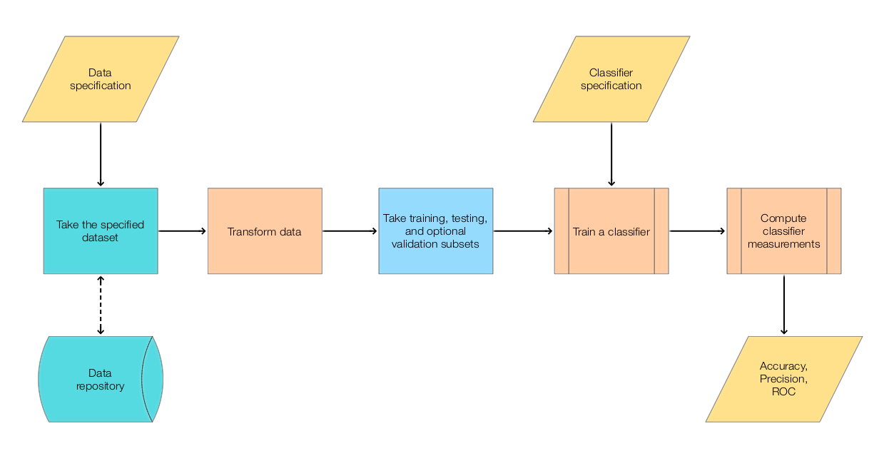
For more details on classification workflows see the article “A monad for classification workflows”. [AA1].

Document execution

This is a “computable Markdown document” – the Raku cells are (context-consecutively) evaluated with the “literate programming” package “Text::CodeProcessing”, [AA2, AAp5].

Remark: This document can be also made using the Mathematica-and-Raku connector, [AA3], but by utilizing the package “Text::Plot”, [AAp6, AA8], to produce (informative enough) graphs, that is “less needed.”

Data

Here we get Titanic data using the package “Data::Reshapers”, [AA3, AAp2]:

use Data::Reshapers;
my @dsTitanic=get-titanic-dataset(headers=>'auto');
dimensions(@dsTitanic)

# (1309 5)

Here is data sample:

to-pretty-table( @dsTitanic.pick(5), field-names => <passengerAge passengerClass passengerSex passengerSurvival>)

# +--------------+----------------+--------------+-------------------+
# | passengerAge | passengerClass | passengerSex | passengerSurvival |
# +--------------+----------------+--------------+-------------------+
# |      40      |      1st       |    female    |      survived     |
# |      20      |      3rd       |     male     |        died       |
# |      30      |      2nd       |     male     |        died       |
# |      30      |      3rd       |     male     |        died       |
# |      -1      |      3rd       |    female    |      survived     |
# +--------------+----------------+--------------+-------------------+

Here is a summary:

use Data::Summarizers;
records-summary(@dsTitanic)

# +---------------+----------------+-----------------+-------------------+----------------+
# | passengerSex  | passengerClass | id              | passengerSurvival | passengerAge   |
# +---------------+----------------+-----------------+-------------------+----------------+
# | male   => 843 | 3rd => 709     | 503     => 1    | died     => 809   | 20      => 334 |
# | female => 466 | 1st => 323     | 421     => 1    | survived => 500   | -1      => 263 |
# |               | 2nd => 277     | 726     => 1    |                   | 30      => 258 |
# |               |                | 936     => 1    |                   | 40      => 190 |
# |               |                | 659     => 1    |                   | 50      => 88  |
# |               |                | 446     => 1    |                   | 60      => 57  |
# |               |                | 260     => 1    |                   | 0       => 56  |
# |               |                | (Other) => 1302 |                   | (Other) => 63  |
# +---------------+----------------+-----------------+-------------------+----------------+

Trie creation

For demonstration purposes let us create a shorter trie and display it in tree form:

use ML::TriesWithFrequencies;
my $trTitanicShort = 
  @dsTitanic.map({ $_<passengerClass passengerSex passengerSurvival> }).&trie-create
  .shrink;
say $trTitanicShort.form;

# TRIEROOT => 1309
# ├─1st => 323
# │ ├─female => 144
# │ │ ├─died => 5
# │ │ └─survived => 139
# │ └─male => 179
# │   ├─died => 118
# │   └─survived => 61
# ├─2nd => 277
# │ ├─female => 106
# │ │ ├─died => 12
# │ │ └─survived => 94
# │ └─male => 171
# │   ├─died => 146
# │   └─survived => 25
# └─3rd => 709
#   ├─female => 216
#   │ ├─died => 110
#   │ └─survived => 106
#   └─male => 493
#     ├─died => 418
#     └─survived => 75

Here is a mosaic plot that corresponds to the trie above:

(The plot is made with Mathematica.)

Trie classifier

In order to make certain reproducibility statements for the kind of experiments shown here, we use random seeding (with srand) before any computations that use pseudo-random numbers. Meaning, one would expect Raku code that starts with an srand statement (e.g. srand(889)) to produce the same pseudo random numbers if it is executed multiple times (without changing it.)

Remark: Per this comment it seems that a setting of srand guarantees the production of reproducible between runs random sequences on the particular combination of hardware-OS-software Raku is executed on.

srand(889)

# 889

Here we split the data into training and testing data:

my ($dsTraining, $dsTesting) = take-drop( @dsTitanic.pick(*), floor(0.8 * @dsTitanic.elems));
say $dsTraining.elems;
say $dsTesting.elems;

# 1047
# 262

(The function take-drop is from “Data::Reshapers”. It follows Mathematica’s TakeDrop, [WRI1].)

Alternatively, we can say that:

We get indices of dataset rows to make the training data
We obtain the testing data indices as the complement of the training indices

Remark: It is better to do stratified sampling, i.e. apply take-drop per each label.

Here we make a trie with the training data:

my $trTitanic = $dsTraining.map({ $_.<passengerClass passengerSex passengerAge passengerSurvival> }).Array.&trie-create;
$trTitanic.node-counts

# {Internal => 63, Leaves => 85, Total => 148}

Here is an example decision-classification:

$trTitanic.classify(<1st female>)

# survived

Here is an example probabilities-classification:

$trTitanic.classify(<2nd male>, prop=>'Probs')

# {died => 0.851063829787234, survived => 0.14893617021276595}

We want to classify across all testing data, but not all testing data records might be present in the trie. Let us check that such testing records are few (or none):

$dsTesting.grep({ !$trTitanic.is-key($_<passengerClass passengerSex passengerAge>) }).elems

# 0

Let us remove the records that cannot be classified:

$dsTesting = $dsTesting.grep({ $trTitanic.is-key($_<passengerClass passengerSex passengerAge>) });
$dsTesting.elems

# 262

Here we classify all testing records (and show a few of the results):

my @testingRecords = $dsTesting.map({ $_.<passengerClass passengerSex passengerAge> }).Array;
my @clRes = $trTitanic.classify(@testingRecords).Array;
@clRes.head(5)

# (died died died survived died)

Here is a tally of the classification results:

tally(@clRes)

# {died => 186, survived => 76}

(The function tally is from “Data::Summarizers”. It follows Mathematica’s Tally, [WRI2].)

Here we make a Receiver Operating Characteristic (ROC) record, [AA5, AAp4]:

use ML::ROCFunctions;
my %roc = to-roc-hash('survived', 'died', select-columns( $dsTesting, 'passengerSurvival')>>.values.flat, @clRes)

# {FalseNegative => 45, FalsePositive => 15, TrueNegative => 141, TruePositive => 61}

Trie classification with ROC plots

In the next code cell we classify all testing data records. For each record:

Get probabilities hash
Add to that hash the actual label
Make sure the hash has both survival labels

use Hash::Merge;
my @clRes = 
do for [|$dsTesting] -> $r {
    my $res = [|$trTitanic.classify( $r<passengerClass passengerSex passengerAge>,  prop => 'Probs' ), Actual => $r<passengerSurvival>].Hash;
    merge-hash( { died => 0, survived => 0}, $res)
}

Here we obtain the range of the label “survived”:

my @vals = flatten(select-columns(@clRes, 'survived')>>.values);
(min(@vals), max(@vals))

# (0 1)

Here we make list of decision thresholds:

my @thRange = min(@vals), min(@vals) + (max(@vals)-min(@vals))/30 ... max(@vals);
records-summary(@thRange)

# +-------------------------------+
# | numerical                     |
# +-------------------------------+
# | Max    => 0.9999999999999999  |
# | Min    => 0                   |
# | Mean   => 0.5000000000000001  |
# | 3rd-Qu => 0.7666666666666666  |
# | 1st-Qu => 0.2333333333333333  |
# | Median => 0.49999999999999994 |
# +-------------------------------+

In the following code cell for each threshold:

For each classification hash decide on “survived” if the
corresponding value is greater or equal to the threshold
Make threshold’s ROC-hash

my @rocs = @thRange.map(-> $th { to-roc-hash('survived', 'died', 
                                                select-columns(@clRes, 'Actual')>>.values.flat, 
                                                select-columns(@clRes, 'survived')>>.values.flat.map({ $_ >= $th ?? 'survived' !! 'died' })) });

# [{FalseNegative => 0, FalsePositive => 156, TrueNegative => 0, TruePositive => 106} {FalseNegative => 0, FalsePositive => 148, TrueNegative => 8, TruePositive => 106} .]

Here is the obtained ROC-hash table:

to-pretty-table(@rocs)

# +---------------+---------------+--------------+--------------+
# | FalsePositive | FalseNegative | TrueNegative | TruePositive |
# +---------------+---------------+--------------+--------------+
# |      156      |       0       |      0       |     106      |
# |      148      |       0       |      8       |     106      |
# |      137      |       2       |      19      |     104      |
# |      104      |       9       |      52      |      97      |
# |       97      |       10      |      59      |      96      |
# |       72      |       13      |      84      |      93      |
# |       72      |       13      |      84      |      93      |
# |       55      |       15      |     101      |      91      |
# |       46      |       19      |     110      |      87      |
# |       42      |       23      |     114      |      83      |
# |       33      |       28      |     123      |      78      |
# |       25      |       36      |     131      |      70      |
# |       22      |       39      |     134      |      67      |
# |       22      |       39      |     134      |      67      |
# |       18      |       40      |     138      |      66      |
# |       18      |       40      |     138      |      66      |
# |       10      |       51      |     146      |      55      |
# |       10      |       51      |     146      |      55      |
# |       4       |       54      |     152      |      52      |
# |       3       |       57      |     153      |      49      |
# |       3       |       57      |     153      |      49      |
# |       3       |       57      |     153      |      49      |
# |       3       |       57      |     153      |      49      |
# |       3       |       57      |     153      |      49      |
# |       3       |       57      |     153      |      49      |
# |       3       |       57      |     153      |      49      |
# |       3       |       60      |     153      |      46      |
# |       2       |       72      |     154      |      34      |
# |       2       |       72      |     154      |      34      |
# |       2       |       89      |     154      |      17      |
# |       2       |       89      |     154      |      17      |
# +---------------+---------------+--------------+--------------+

Here is the corresponding ROC plot:

use Text::Plot; 
text-list-plot(roc-functions('FPR')(@rocs), roc-functions('TPR')(@rocs),
                width => 70, height => 25, 
                x-label => 'FPR', y-label => 'TPR' )

# +--+------------+-----------+-----------+-----------+------------+---+        
# |                                                                    |        
# +                                                        *    *  *   +  1.00  
# |                                                                    |        
# |                                         * *                        |        
# |                        *      *                                    |        
# |                    *                                               |        
# +                   *                                                +  0.80  
# |               *                                                    |        
# |                                                                    |        
# |            *                                                       |        
# |         * *                                                        |       T
# +                                                                    +  0.60 P
# |      *                                                             |       R
# |    *                                                               |        
# |   *                                                                |        
# +   *                                                                +  0.40  
# |                                                                    |        
# |   *                                                                |        
# |                                                                    |        
# |                                                                    |        
# +                                                                    +  0.20  
# |   *                                                                |        
# |                                                                    |        
# +--+------------+-----------+-----------+-----------+------------+---+        
#    0.00         0.20        0.40        0.60        0.80         1.00       
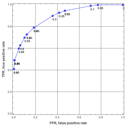
#                                  FPR

We can see the Trie classifier has reasonable prediction abilities – we get ≈ 75% True Positive Rate (TPR) with relatively small False Positive Rate (FPR), ≈ 20%.

Here is a ROC plot made with Mathematica (using a different Trie over Titanic data):

Improvements

For simplicity the workflow above was kept “naive.” A better workflow would include:

Stratified partitioning of training and testing data
K-fold cross-validation
Variable significance finding
Specifically for Tries with frequencies: using different order of variables while constructing the trie

Remark: K-fold cross-validation can be “simply”achieved by running this document multiple times using different random seeds.

References

Articles
[AA1] Anton Antonov, “A monad for classification workflows”, (2018), MathematicaForPrediction at WordPress.
[AA2] Anton Antonov, “Raku Text::CodeProcessing”, (2021), RakuForPrediction at WordPress.
[AA3] Anton Antonov, “Connecting Mathematica and Raku”, (2021), RakuForPrediction at WordPress.
[AA4] Anton Antonov, “Introduction to data wrangling with Raku”, (2021), RakuForPrediction at WordPress.
[AA5] Anton Antonov, “ML::TriesWithFrequencies”, (2022), RakuForPrediction at WordPress.
[AA6] Anton Antonov, “Data::Generators”, (2022), RakuForPrediction at WordPress.
[AA7] Anton Antonov, “ML::ROCFunctions”, (2022), RakuForPrediction at WordPress.
[AA8] Anton Antonov, “Text::Plot”, (2022), RakuForPrediction at WordPress.
[Wk1] Wikipedia entry, “Receiver operating characteristic”.
Packages
[AAp1] Anton Antonov, Data::Generators Raku package, (2021), GitHub/antononcube.
[AAp2] Anton Antonov, Data::Reshapers Raku package, (2021), GitHub/antononcube.
[AAp3] Anton Antonov, Data::Summarizers Raku package, (2021), GitHub/antononcube.
[AAp4] Anton Antonov, ML::ROCFunctions Raku package, (2022), GitHub/antononcube.
[AAp5] Anton Antonov, Text::CodeProcessing Raku package, (2021), GitHub/antononcube.
[AAp6] Anton Antonov, Text::Plot Raku package, (2022), GitHub/antononcube.
[AAp7] Anton Antonov, ML::TriesWithFrequencies Raku package, (2021), GitHub/antononcube.
Functions
[WRI1] Wolfram Research (2015), TakeDrop, Wolfram Language function, (updated 2015).
[WRI2] Wolfram Research (2007), Tally, Wolfram Language function.
Here is a notebook making more or less the same computations in Mathematica : https://community.wolfram.com/groups/-/m/t/2605320 .